How To: Simulate Glass Transition Temperature for Curing Process

Curing of epoxy resin with diffusion control

Example for this Guide

Find glass transition temperature Tg as the function of time and coordinate for the curing process of epoxy in the cylindrical container.

1. Introduction

The temperature of glass transition is very important property of the material and has influence on its the physical and chemical properties. However, it changes during the curing reactions of thermosets. For the cured product the glass transition temperature is higher than for the uncured reactant. In the large, industrial volumes with temperature gradients, where temperature and degree of cure depends on coordinates, the glass transition temperature and physical properties are coordinate-dependent too.

In the current guide we will show how to simulate the curing process for epoxy resin for the cylindrical volume, including the coordinate-dependent glass transition temperature at each time point.

As basis we will use the pre-installed sample: Kinetics Neo project DSC_Diff_Control_Epoxy_Analysis.kinx2. This project contains the diffusion controlled curing of epoxy, which is described in the guides in Learn section of our Kinetics Neo web site:

How To: DSC Curing, Data for Diffusion Control - NETZSCH Kinetics Neo

For material in this guide the glass transition temperature changes from 25°C (uncured material) to 165°C (completely cured material).

Now we will simulate, how the glass transition temperature changes during the curing process in the large volume.

2. Create New Project in Termica Neo

Start Termica Neo.

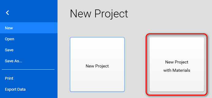
In the main ribbon of the top of the Termica Neo main window select File - New - New Project with Materials:

Please save your just created project file.

3. Create Reactant

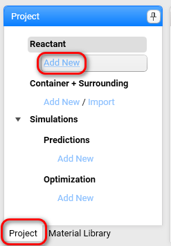
On Project Panel click on Add New in Reactant section:

Set physical properties for reactant: Select Epoxy from drop down list in section Physical Properties:

Now the following temperature-dependent physical properties of the reactant are filled:

Specific heat,
Density,
Thermal conductivity.

In the section Kinetics Data select Kinetics Neo project with chemical kinetic properties of the selected material.

Click on Import Kinetics Neo Project File.

In the File Open dialog go to the folder C:\Users\Public\Documents\NETZSCH\Termica Neo\Samples\Epoxy_Diffusion_Control .

In this folder select the DSC_Diff_Control_Epoxy_Analysis.kinx2 file:

Kinetics Neo project will be loaded. Now we need to select a correct kinetics model in it to use in our guide.

In the list Kinetics Model and Methods select s:; Cn diff model. The kinetics simulation chart will be loaded:

4. Create Container and Surrounding

Now we will create new Container and Surrounding and fill their properties. Details about Container and Surrounding can be found in Projects Structure.

On Project Panel select Add New in Container + Surrounding section:

Type container Name: Epoxy_Cylinder.

Select Cylinder from drop-down for container shape.

Set properties for Reactant Dimensions:

Radius: 10 cm

Height: 8 cm

Set following properties for Container Surfaces:

Surface: S1 Top:

Material: Aluminium
Thickness: 0.3 cm
Surrounding: Air

Surface: S2 Side:

Material: Aluminium
Thickness: 0.5 cm
Surrounding: Water (no moving)

Surface: S3 Bottom

Material: Aluminium
Thickness: 1 cm
Surrounding: Water (no moving)

After all changes we will finish configuring the container and surfaces properties:

5. Create Prediction

On Project Panel select Add New for Predictions item in Simulations section:

Fill Prediction Name: Prediction_Epoxy - Diff .

Select Epoxy Diff from drop-down list for Reactant:

The kinetic method for this reactant is shown in the Method field. It can be changed in Reactant section.

Set Enthalpy and Initial Temperature:

For kinetic project based on DSC data, the enthalpy values are taken directly from kinetic project. Therefore we recommend not to change it.

Initial Temperature should be set to your initial conditions. Set it to 25 °C:

Select Epoxy_cylinder from the Container drop-down list:

Set the Surrounding conditions.

For this sample we will use different temperature conditions for all three surfaces. Select check box Different Surroundings for all surfaces. The surrounding conditions for all three surfaces will be shown.

Set the following surrounding conditions:

Surface: S1 Top

Temperature profile: Isothermal
Temperature: 25 °C
Time: 100 min

Surface: S2 Side

Temperature profile: Isothermal
Temperature: 100 °C
Time: 100 min

Surface: S3 Bottom

Temperature profile: Isothermal
Temperature: 120 °C
Time: 300 min

Here you see, that we use isothermal temperature profile for all surfaces, but these profiles have different time: time 100 minutes for top and side surfaces and time 300 for bottom surface.

If the temperature programs for different surfaces have different duration, then the predictions will be done for the longest time duration. The temperature profiles for other surfaces with the shorter time duration will be extended to the longest duration by adding of isothermal segment at the end, to have the same duration as the longest segment. The temperature of this additional isothermal segment is set to be equal to the temperature of the last point of this short temperature profile.

Details: 4.1 Create Simulation Prediction (termica.help), section 4.1.7

Click on Calculate to perform simulation. Depending on you computer hardware, the calculation can take some time. In this case you will see progress bar indicating the calculation progress:

Please be patient and wait until calculation finishes:

When the calculation finishes, the simulation chart will be shown on the right panel.

The calculation time is shown on the bottom of the Properties panel under the button Calculate. It will differ for different computers. It depends also from the Accuracy Level setting (for details read about 3D Accuracy Level setting in 7. Settings in termica.help)

6. Simulation Results for Tg

Select the Tg (Glass) in the Y-Axis group in Ribbon toolbar and the glass transition temperature will be shown:

It could be also shown in 3D view as the function of coordinate and time.

Select 3D in Chart Type group in the top left of the main Ribbon:

You can rotate the 3D chart by holding the left mouse key and moving the mouse.

You can zoom the chart by just rotating the mouse wheel.

You can also move the 3D chart inside the plot area by holding the right mouse key and moving the mouse. Chart will move to the direction opposite to moving the mouse.

Alternatively, it could be shown as Tg for the vertical or horizontal cross-section.

Select Section in Chart Type group in the top left of the main Ribbon. Section chart as function of 2 coordinates X and Y will be shown:

Initially the Time Frame 0 seconds will be set.

Move slider below the Time Frame value to change it. The chart will be changed to show the simulation for selected time frame.

It is also possible to set exact value of the time frame in the corresponding text box. Set value 139 seconds there and click on OK button:

The Section 3D Chart can be also rotated by holding the left mouse key and moving the mouse:

3D chart can be also shown as Heatmap chart.

Select Heatmap in 3D / Section group in the top left of the main Ribbon. Heatmap chart will be shown.

Select Keep Aspect Ratio check box to keep the same size for both dimensions X and Y:

Section 3D and Heatmap charts can be shown not only in axial (default) plane like all figures before, but also in radial plane. To switch plane select Radial option in Plane group of main ribbon. We will get the Heatmap chart in radial projection of the cylinder container:

If plane is set to Radial then it is possible to see the simulations on different heights of our cylinder. To change the default value z = 50% please move the vertical slider in the Plane group of main ribbon. Below are the results for z = 20%, 50%, 80%:

Z = 80%