
Termica Neo: First Steps
Creating a new project in Termica Neo from the beginning to final simulations
Termica Neo is software for the simulation of thermal behavior for chemical reactions and crystallization in solids or liquids, in volumes with linear sizes from centimeters to meters. The main applications are chemical processes in materials with high thermal potential, as well as reactions involving curing, cross-linking, sintering and polymer crystallization.
In this guide, we will follow these steps from the very beginning to create a simulation at the end.
Example for this Guide
Find the degree of cure for epoxy curing in an infinite cylinder of diameter D = 20 cm with an aluminum container of 1 cm thickness as the function of time at a given radial coordinate
1. Start Termica Neo Software
Just start Termica Neo software on your computer.
2. Create Project
In the main ribbon of the top of the main window, select File - New - New Project with Materials:
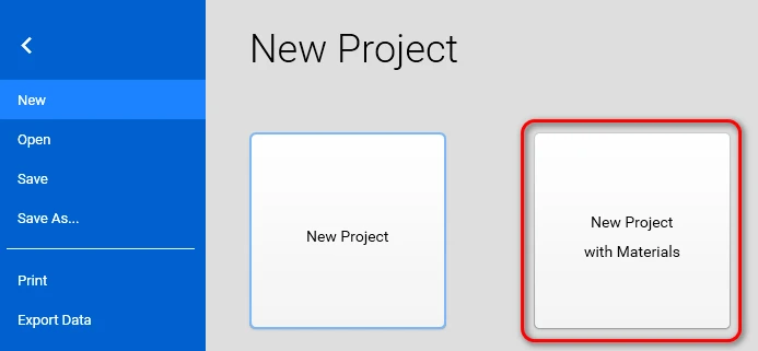
The new project is created and contains several predefined materials in Material Library.
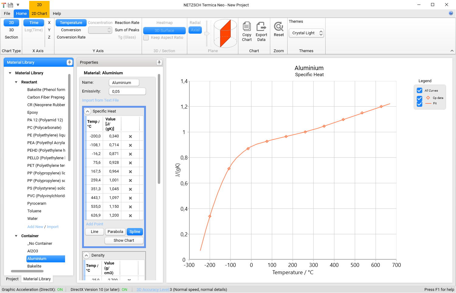
Please click on the Material Library tab on the bottom in order to check that the library is filled. You can select any material in the left panel and see the temperature-dependent physical properties on the chart.
Here, the Aluminium container material is selected, and it contains the physical properties of specific heat, density, thermal conductivity.
Save your project under the new name MyFirstProject.tsimx using menu File - Save As … .
3. Create Reactant
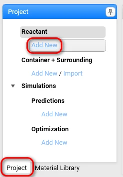
3.1 On the Project panel, click on Add New in the Reactant section:
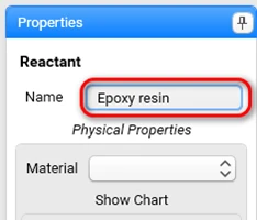
3.2 Fill in the reactant name Epoxy resin instead of <new reactant>:
3.3 Set the physical properties for Reactant: Select Epoxy from the drop-down list in the section Physical Properties:
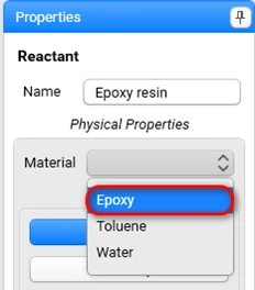
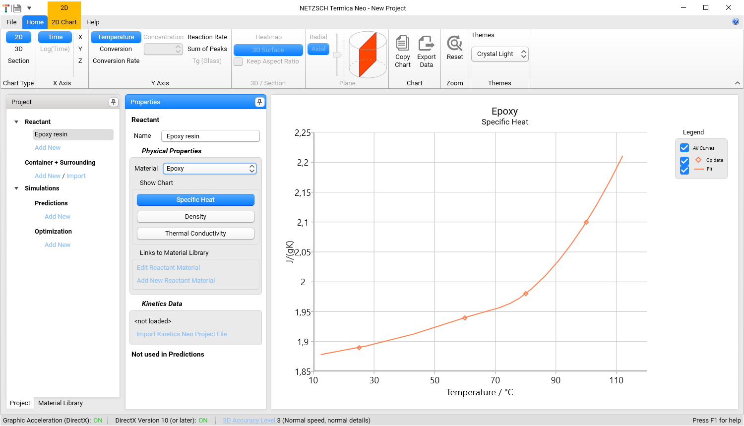
Now the following temperature-dependent physical properties of the reactant are filled in:
- Specific heat,
- Density,
- Thermal conductivity:
3.4 Set chemical properties for Reactant:
In the section Kinetic Data click on Import Kinetics Neo Project File, and in the folder:
C:\Users\Public\Documents\NETZSCH\Termica Neo\Samples\1_FirstProject
... select the file DSC_Kinetics_Epoxy.kin2x . The kinetics model is loaded from the kinetic project.

If the kinetic project contains several kinetic evaluations, including model-free methods and different kinetic models, then all of them are loaded into the Termica Neo project and you will be able to select here the best one for use in the simulations.
Additional information about the Reactant can be found in Projects Structure.
4. Create Container and Surrounding
Now we will create a new Container and Surrounding and fill in their properties. Details about the Container and Surrounding can be found in Projects Structure.
4.1 On the Project panel, select Add New in the Container + Surrounding section.

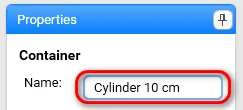
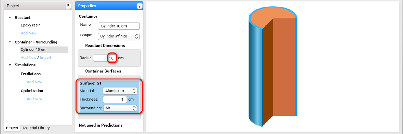
4.2 Fill in the container Name: Cylinder 10cm.
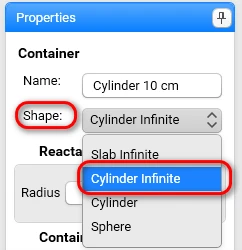
4.3 Select Cylinder Infinite from the drop-down for container shape.
4.4 Set the Reactant Dimension:
- Radius: 10 cm
4.5 Set properties for Container Surfaces:
- Material: Aluminum
- Thickness: 1 cm
- Surrounding: Air
If the shape of the container is complex, then different surfaces may have different walls of different materials and thicknesses. Additional information about Container and Surrounding can be found in Projects Structure.
5. Create Prediction
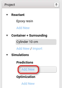
5.1 On the Project panel, select Add New for the Predictions item in the Simulations section:
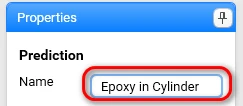
5.2 Fill in Prediction Name: Epoxy in Cylinder.
5.3 Select Epoxy resin from the drop-down list for Reactant:
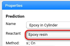
The kinetic method for this reactant is shown in the Method field. It can be changed in the Reactant section.
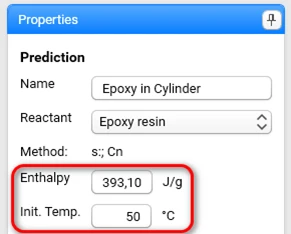
5.4 Set Enthalpy and Initial Temperature:
For a kinetic project based on DSC data, the enthalpy values are taken directly from the kinetic project. Therefore we recommend not to change it.
Initial Temperature should be set to your initial conditions. Set it to 50 °C:
5.5 From the Container drop-down list, select Cylinder 10 cm :

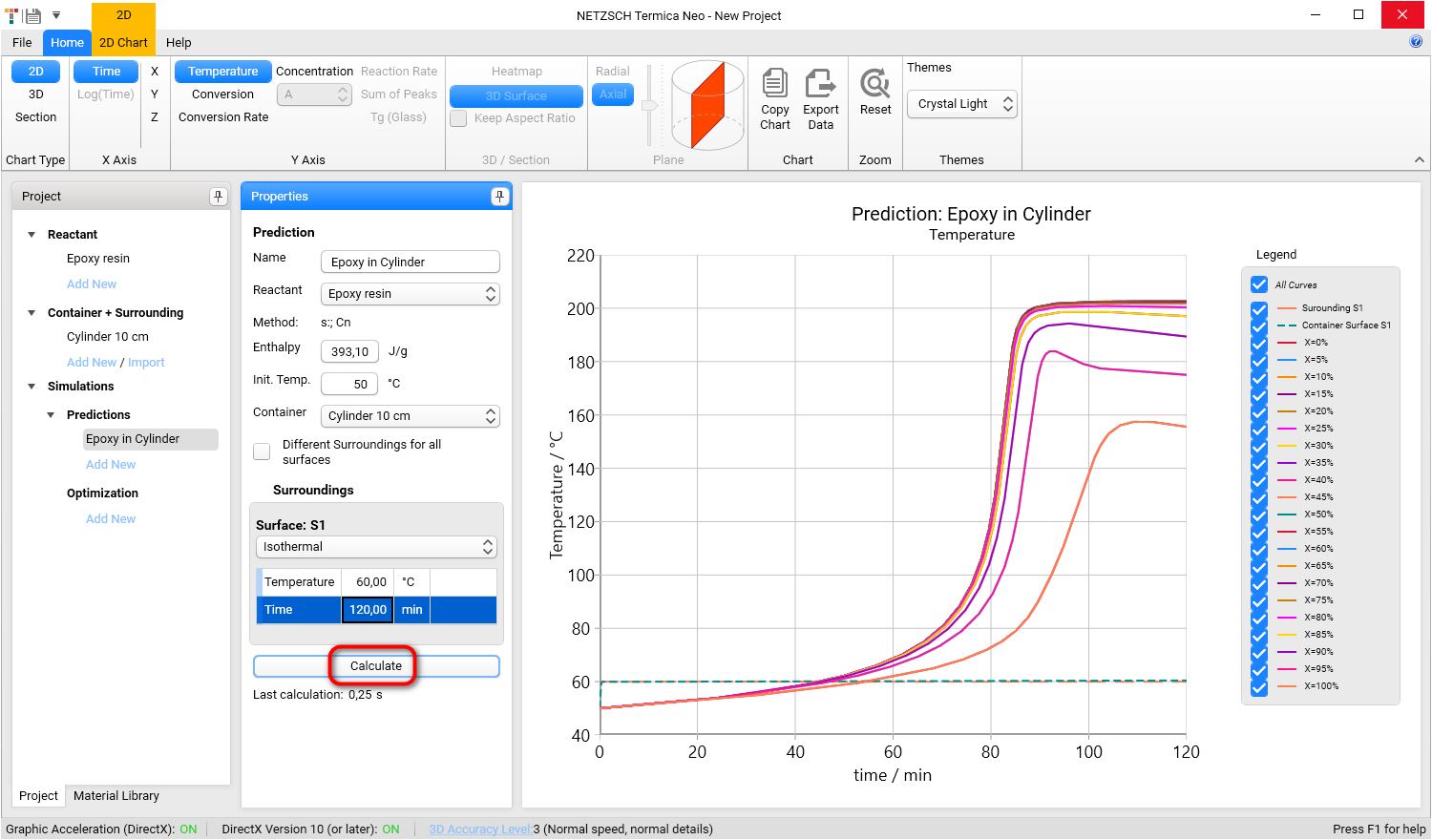
5.6 Set Temperature conditions for environments in the Surroundings section:

5.7 Click on Calculate to perform the simulation:
Additional information about Simulations can be found in Simulations.
6. Simulations
Now we will look at the simulation results using different charts.
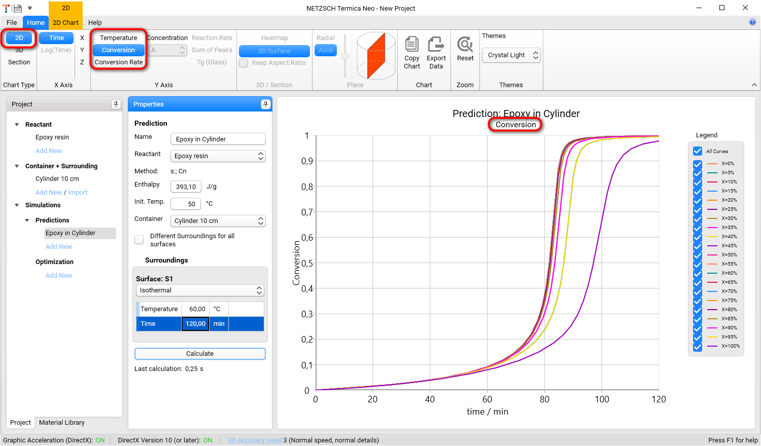
6.1 Temperature, conversion or conversion rate as the time-dependent 2D curves at different coordinates:
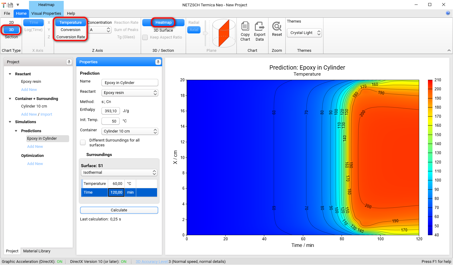
6.2 Signal as a function of X and time in the view of 3D Heatmap:
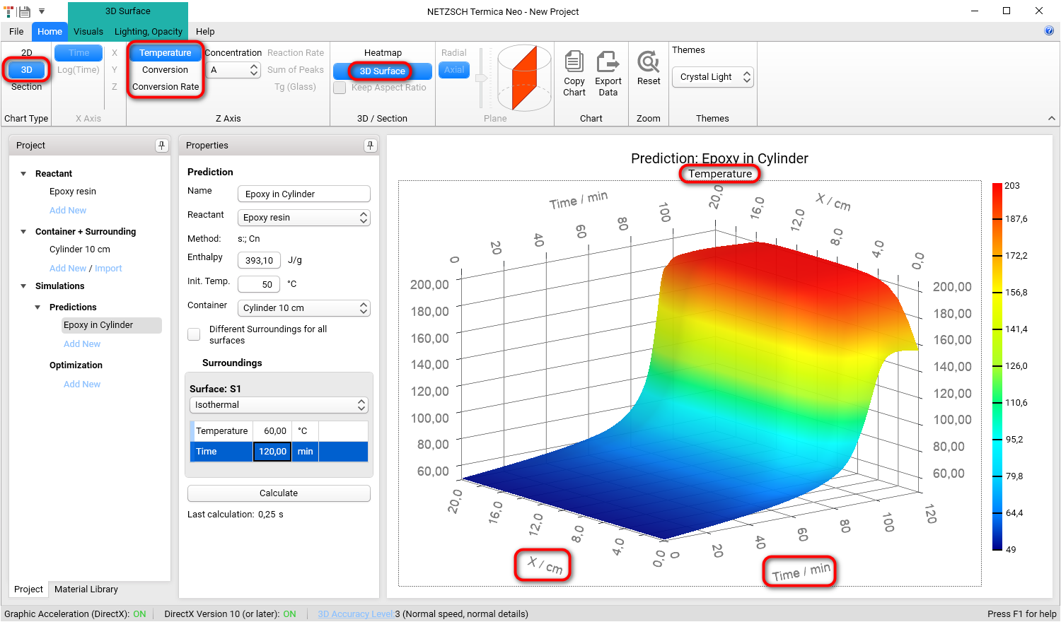
6.3 Signal (temperature, conversion or conversion rate) as a function of X and time in the view of 3D Surface:
6.4 Signal for cross-section in the view of 3D Heatmap at the selected time point:
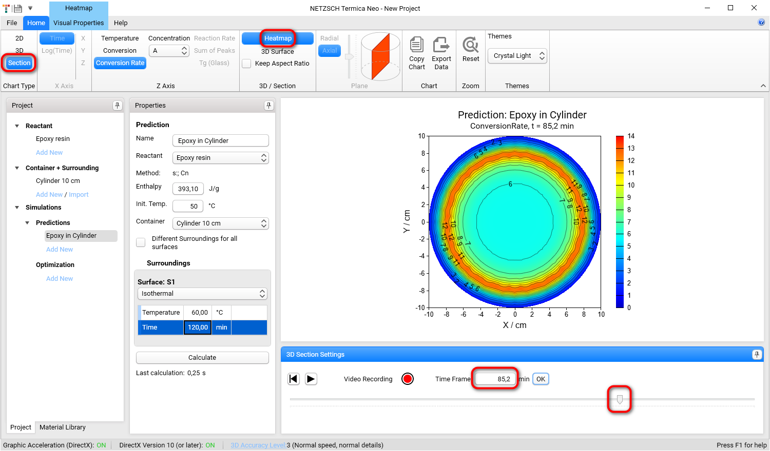
Please move the slider at the bottom right in order to select the time point.
6.5 Signal for cross-section in the view of 3D Surface at the selected time point

7. Create Optimization: SADT
7.1 Create new Optimization
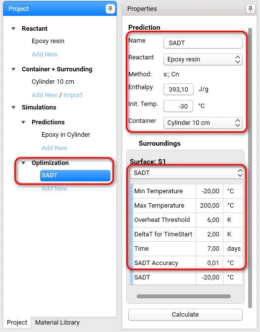
In the Project tree, go to Optimization and click on the Add New link. A new optimization will be created.
Set the optimization's name to SADT and fill in its parameters as seen in the screenshot:
7.2 Calculate SADT
Calculate the SADT for the given parameters by clicking on Calculate.
The Self-accelerating Decomposition Temperature is calculated for the given parameters and it is shown in the last row of the parameter table:

Here, for faster calculation, the Accuracy Level was set to 2 (default: 3). For details about Accuracy Level, see 7. Settings (termica.help) , section 7.4 Accuracy Level.