How To: Simulate Individual Concentrations

Example for this Guide

Find the concentrations of initial reactant, intermediate reactant, and final product as the functions of time and coordinate for the multi-step decomposition of polymer in spherical container.

Contents

1. Introduction

2. Load the Sample Data Project

3. Select Multi-Step Reaction Model for Reactant

4. Select Container and Surrounding

5. Simulation and Results

5.1 Simulate Prediction

5.2. Concentrations as 2D Curve

5.3 Concentration of Selected Reactant in Section View as Heatmap Chart

5.4. Concentration of Selected Reactant as a Function of Time and Spatial Coordinate

1. Introduction

The multi-step reactions contain individual reaction steps and the intermediate reactants. The concentration of intermediate reactants increases during those steps where they are the products. Then the concentration of intermediate reactants decreases in the steps where they are reactants. For some processes it is very important to know how the concentrations of the reactants, including intermediate reactants, depends on coordinate during the process.

In this guide we will show how to simulate the concentrations of all reactants, including intermediate reactants, during multi-step decomposition process, and how to present the coordinate- and time-dependent results.

2. Load the Sample Data Project

Start Termica Neo software.

Click on the File tab on the top left of Termica Neo window to open the application menu.

In the application menu click on Open. An Open Project panel will be shown:

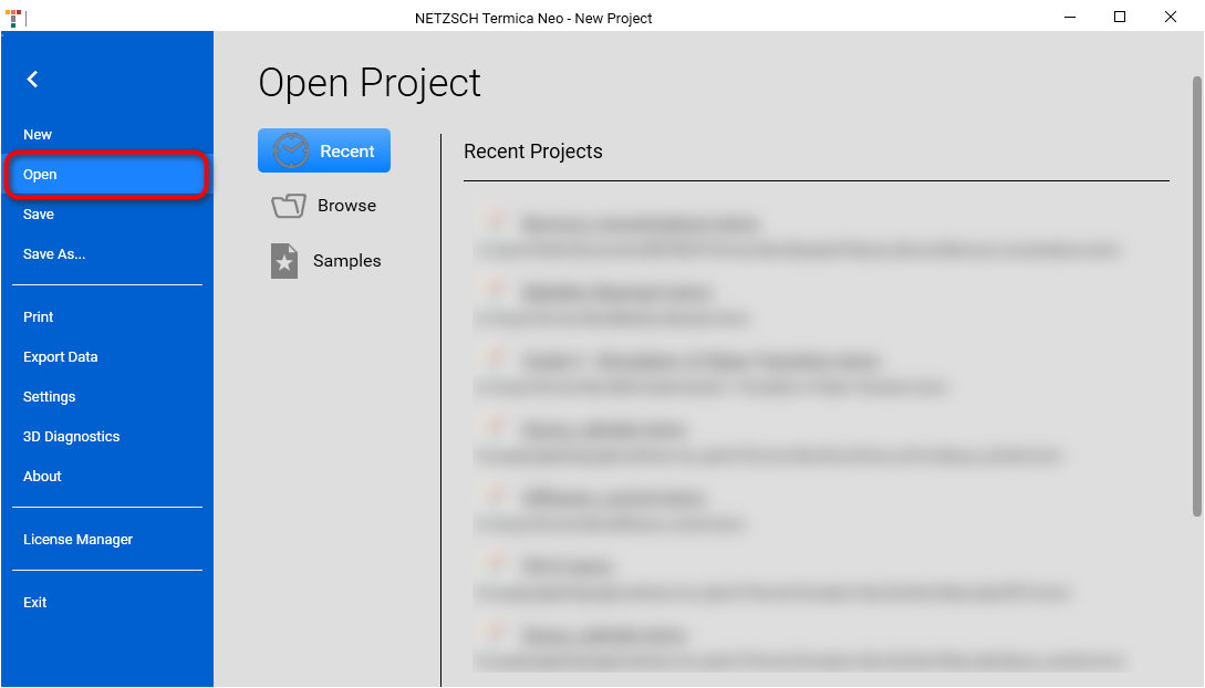
In the Open Project panel click on Samples button. The File Open dialog will be shown and the local file folder C:\Users\Public\Documents\NETZSCH\Termica Neo\Samples will be loaded. Our sample is located in the folder Polymer_Burnout:

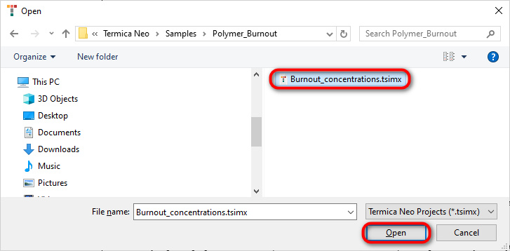
Open folder folder Polymer_Burnout. In this folder open the file Burnout_concentrations.tsimx:

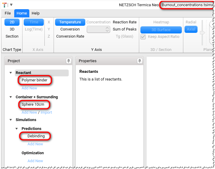
The Burnout_concentrations.tsimx project will be loaded:

3. Select Multi-Step Reaction Model for Reactant

It is important for this guide to select a multi-step reaction model to get simulation of concentration for different reactants. 

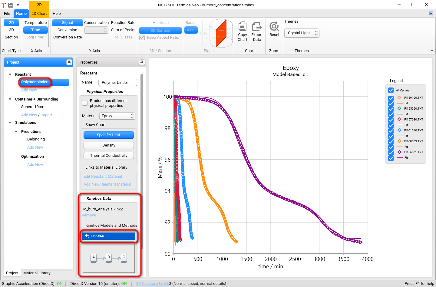
In Project panel on the left select reactant Polymer binder.

In the Properties panel scroll down to the section Kinetics Data and ensure that multi-step kinetic model d: is selected:

4. Select Container and Surrounding

In Project panel select Sphere 10 cm under Container + Surrounding and ensure that the spherical container with radius 10 cm is selected.

5. Simulation and Results

5.1 Simulate Prediction

Now we will prepare and calculate the simulation of temperature for spherical container with Radius 10 cm. 

In In Project panel on the left select Debinding under Simulations / Predictions. Check the values on the Properties panel.

Click on the button Calculate.

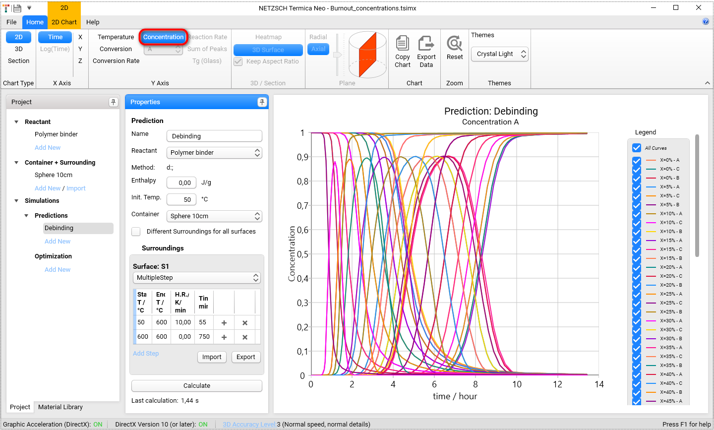
5.2. Concentrations as 2D Curve

Select the concentrations in X-Ais group on the ribbon toolbar. For 2D-view all individual reactants (A,B,and C) can be shown at each point.

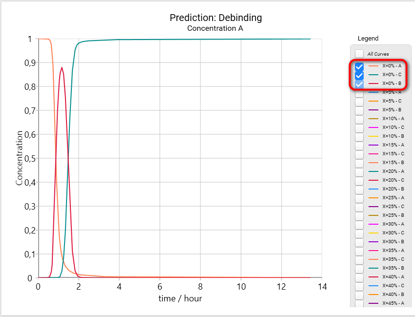
Let's have a look on the concentration of all three reactants in coordinate X = 0 (X=0%). This corresponds to the surface of our sphere. In Legend switch off check box All Curves and select first three curves only:

• X=0% - A
• X=0% - C
• X=0% - B

To show the simulated concentrations in the center of our spherical container please clear previous selection and select :

• X=50% - A
• X=50% - C
• X=50% - B

Maybe you will need to scroll the legend to see the 50% curves.

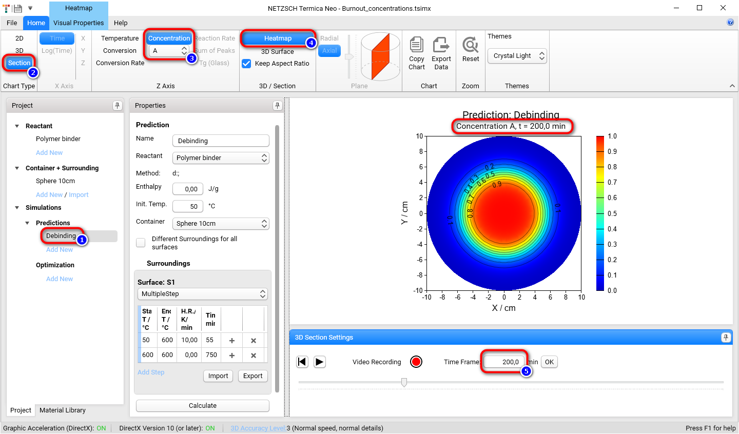
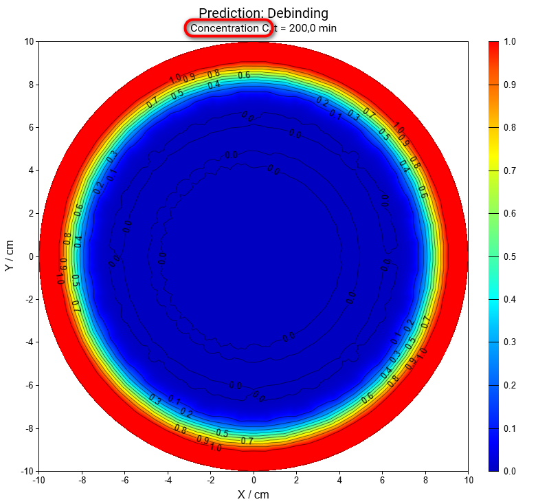
5.3 Concentration of Selected Reactant in Section View as Heatmap Chart

In Cross-section view the only one selected concentration can be shown. 

1. We are still use Debinding prediction in Termica Neo.
2. In the main ribbon please select Section in the group Chart Type.
3. In the ribbon in the group Z-Axis check that Concentration is selected and Reactant A is selected from drop-down list.
4. Select Heatmap view.
5. In the 3D Section Properties panel in the bottom right part of the main window set Time Frame value to 200 minutes and click on OK button.

Now we will have a look at the simulation of concentration for each 3 reactants:

Reactant A by 200 minutes (same settings as above), large image:

Select reactant B from Concentration Reactants drop-down menu on the main ribbon:

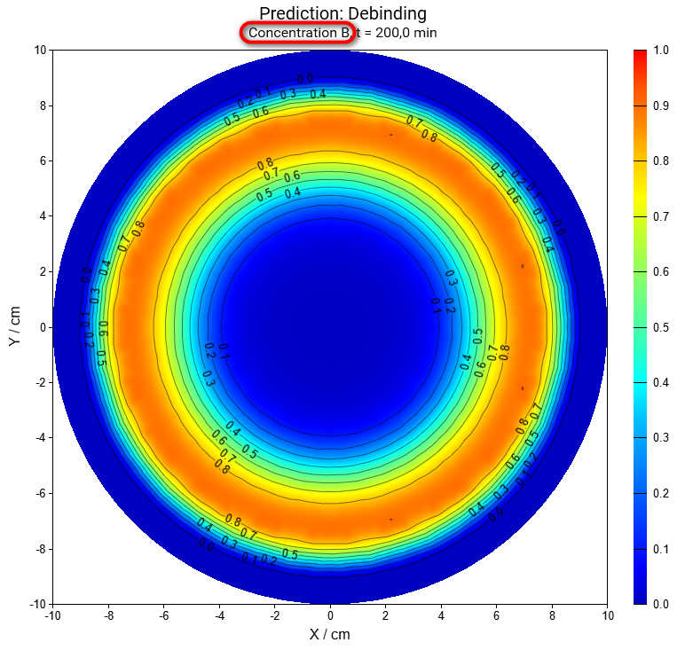
Same for concentration of reactant C:

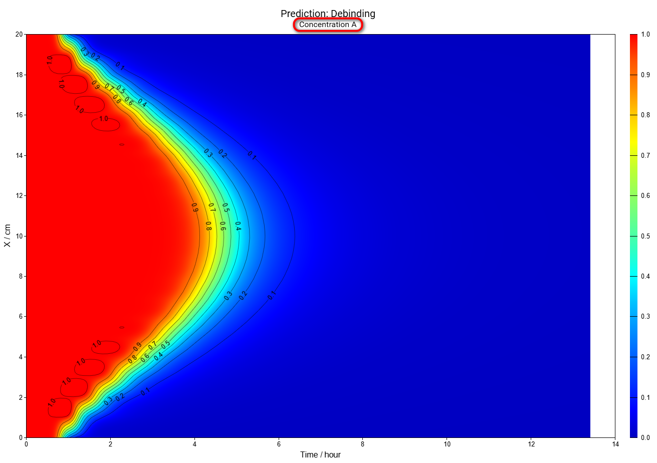
5.4. Concentration of Selected Reactant as a Function of Time and Spatial Coordinate

Now we will show the results of simulation concentrations of A,B and C as the function of coordinate and time. Please switch Chart Type from Section to 3D.

Please also select reactant A from the Concentration Reactants drop-down menu on the main ribbon.

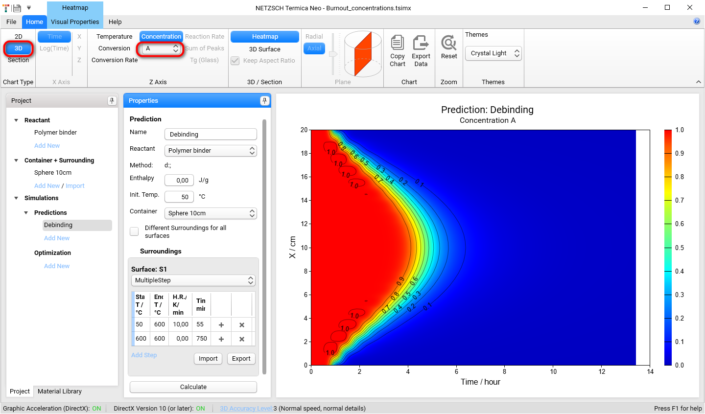
Now we will have a look at the simulation of concentration for each 3 reactants:

Reactant A by 200 minutes (same settings as above), large image:

Select reactant B from Concentration Reactants drop-down menu on the main ribbon:

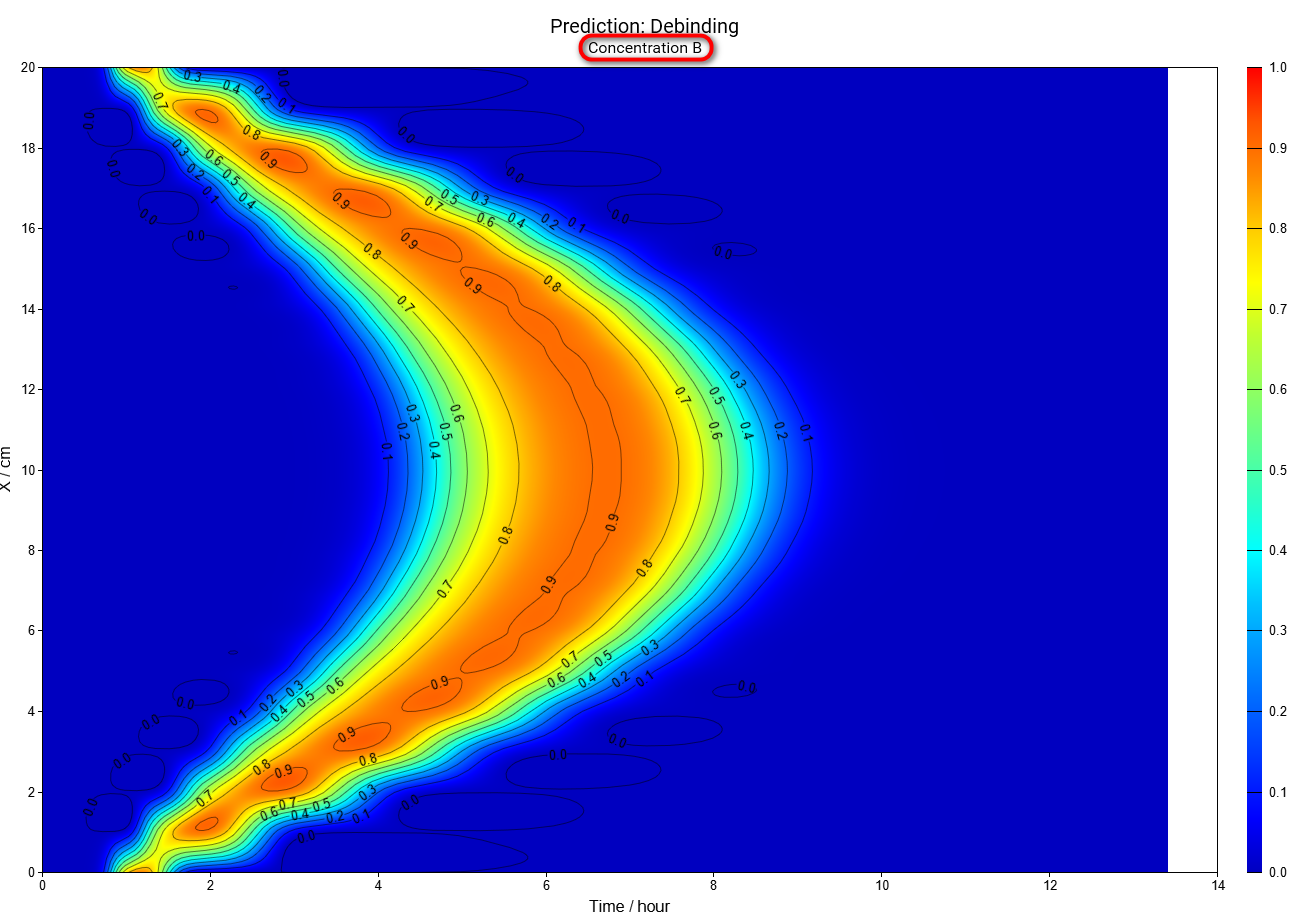
Same for concentration of reactant C:

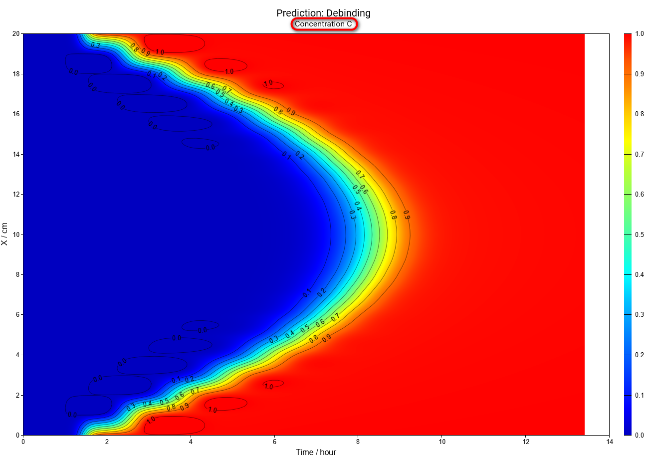
In this simulation we can see that the intermediate reactant B has the maximal concentration in the center after 7 hours, but near the surface the maximum is after 1.1 hours only.